6 Customer Growth & Cohort Retention
6.1 A Shrinking Pipeline
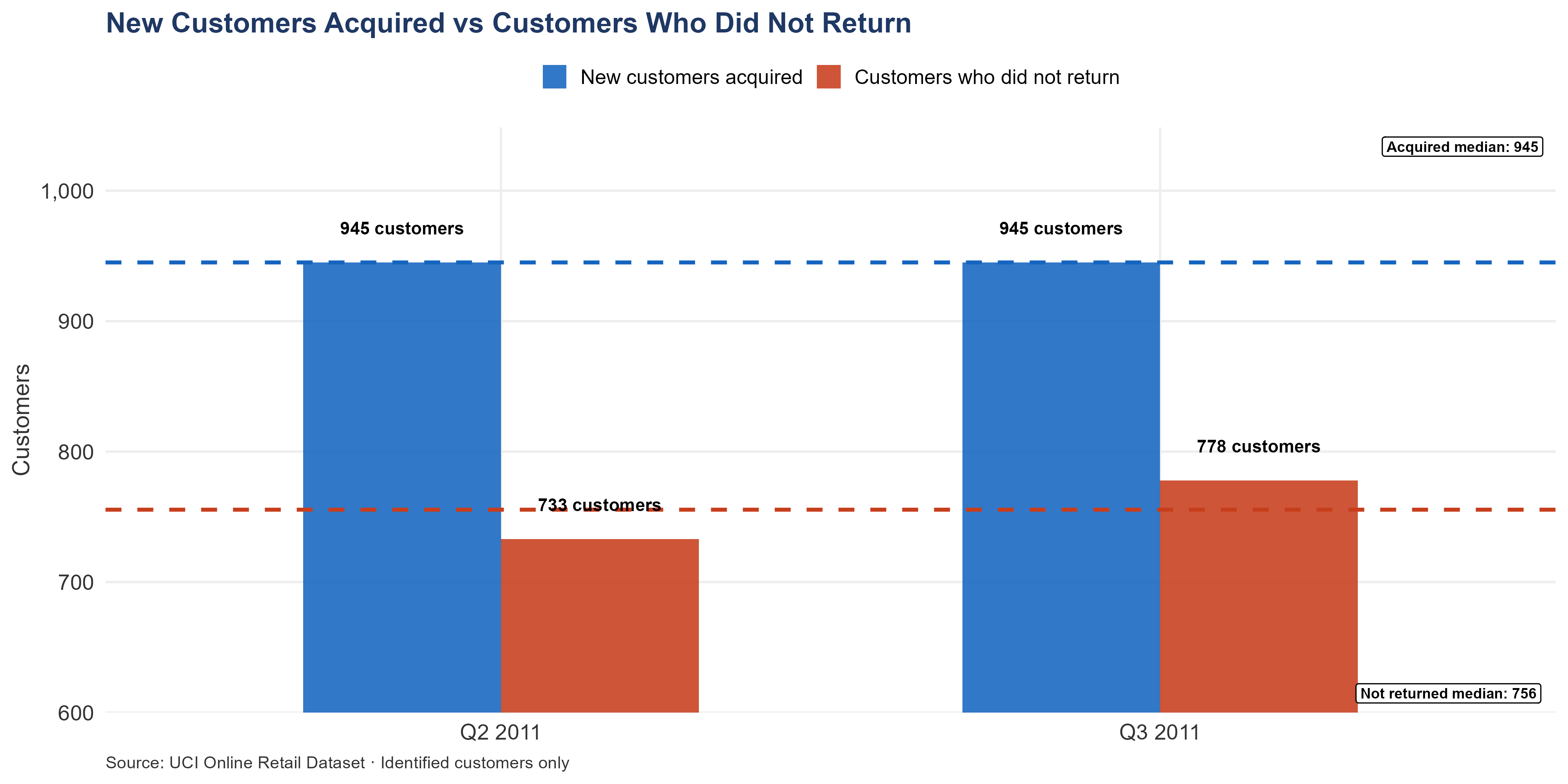
New customer acquisition has been declining for most of 2011. In the UK, the number of new customers dropped from 419 in March to just 141 in August — a 66.35% fall over five months. While Q4 brought a partial recovery, it never reached Q1 levels. The Q3 group of new customers is 47.63% smaller than Q1.
This matters because the revenue growth that makes the second half of 2011 look so attractive was driven almost entirely by returning customers, not new ones. The business is drawing from a shrinking well. For a prospective buyer, projecting 2012 revenue based on the H2 2011 trajectory is risky — it builds a model on an acquisition pipeline that no longer exists at the same scale.
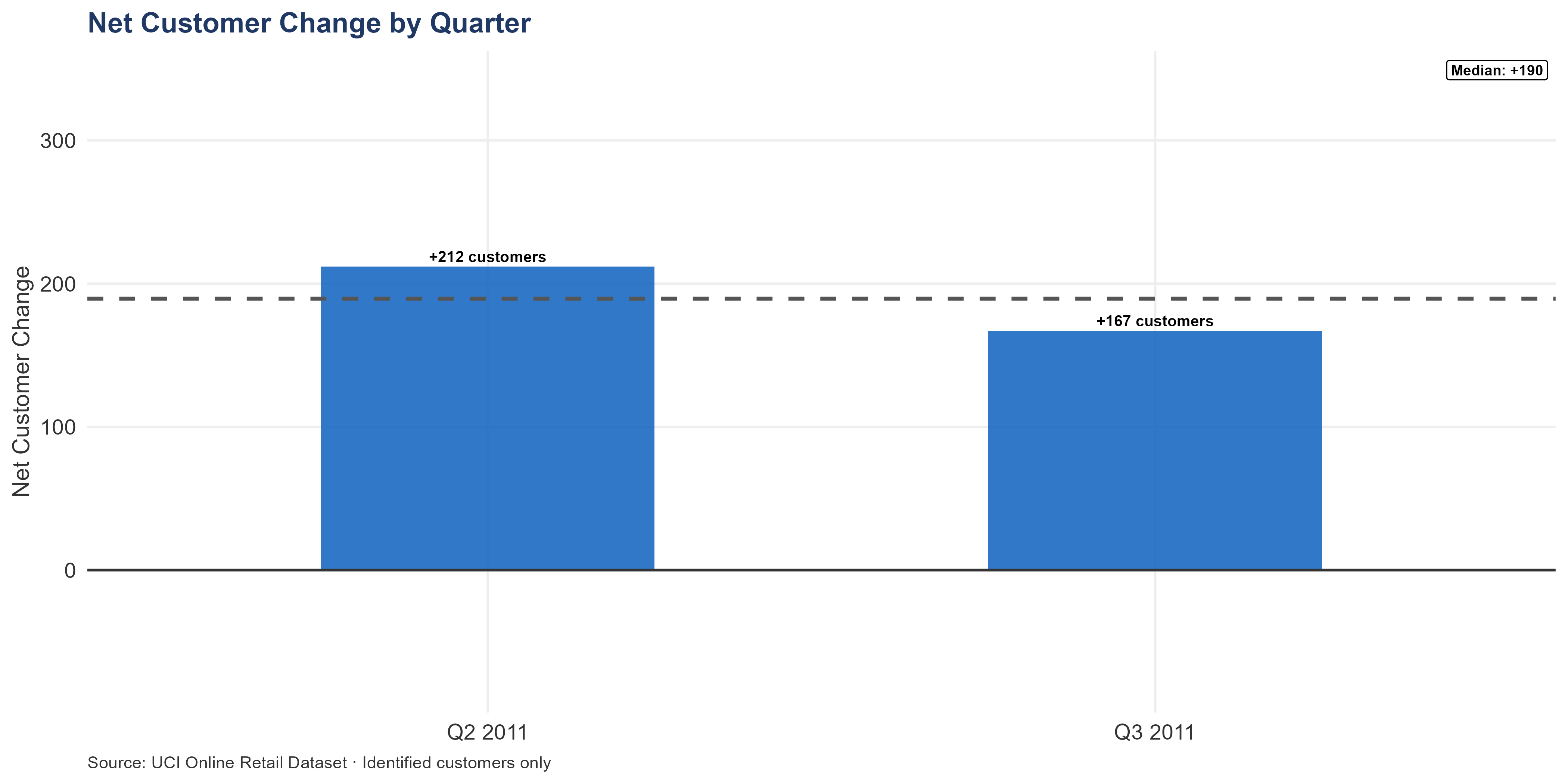
If returning customers are growing, a dip in new acquisitions is manageable. If not, it is a significant revenue risk.
6.2 First-Order Retention — The Repeat Purchase Rate
Do customers come back after their first order? The short answer is yes — most of them do, given enough time.
The numbers look alarming at first glance. Among customers acquired in Q1 2011, 69.3% eventually returned. By Q2, that figure drops to 52.4%. By Q3, just 21.8%. It looks like the business is hemorrhaging customers at an accelerating pace.
It is not. The real explanation is far more mundane: later customers simply had less time to come back before the observation window closed. Q1 customers had nine months of runway. Q3 customers had barely three — not even enough for two full ordering cycles at the typical seven-week gap between orders. When you compare apples to apples — looking only at the first quarter after acquisition — the drop is real but modest: about 50% for Q1, about 42% for Q2.
The important takeaway is what the data does not show. There is no sign that customers are actively choosing to leave. When given enough time, the majority return. The business is not losing customers to dissatisfaction. It is losing them to silence — nobody is reaching out during the window when a nudge would bring them back.
6.3 The December 2010 Baseline
One group of customers stands apart from all the others: those acquired in December 2010. They are the only cohort with a full year of data — every other group’s track record is cut short by the dataset’s December 9, 2011 cutoff.
The results are remarkable. Out of 884 customers who first ordered in December 2010, 87% came back for a second order within a year. Their spending grew steadily over time: £529 per customer after three months, £875 after six, £1.10K after nine, and £1.64K after a full year. These are customers who kept buying more as the relationship matured.
One caveat worth noting: December is the busiest month of the year. Customers drawn in during the holiday rush might behave differently from those acquired in quieter periods — some may have been seasonal shoppers or bargain hunters rather than long-term wholesale accounts. So while 87% is the most reliable retention number in this entire analysis, it might paint a slightly rosier picture than what a typical month produces.
That said, this is the yardstick. Every 2011 cohort is measured against it. When a 2011 group comes close to this number, it suggests their lower raw figures are just a data-window issue. When they fall well short, something more concerning may be at play.
6.4 Q1 2011 — The Biggest Group, and the Biggest Question Mark
The first quarter of 2011 brought in more new customers than any other period: 1,248 of them, nearly half again as many as the next-largest quarter. By sheer numbers, this group will dominate the business’s revenue picture heading into 2012. More of next year’s returning customers will come from Q1 2011 than from any other source.
Here is the problem: this same group also had the highest rate of customers who ordered once and never came back. About 69% of Q1 2011 customers — those with enough time to have reasonably returned — placed a single order and disappeared.
Largest intake, worst retention. That combination demands an explanation, and two plausible ones exist side by side.
The first is a timing issue. Q1 customers had at most nine months before the dataset’s December 9 cutoff. Anyone whose natural buying rhythm falls on a ten-, eleven-, or twelve-month cycle would look like a lost customer even though they were always planning to come back. If this is what happened, the real retention rate is much better than it appears — and the 2012 returning-customer pool from this group will be large and valuable.
The second is a quality issue. Something about Q1 acquisition — a promotion, a new advertising channel, a pricing experiment — may have attracted customers who were never likely to become regulars. If this is even partly true, the business spent its biggest acquisition quarter bringing in people who had no intention of sticking around.
This dataset alone cannot resolve which explanation is correct. But a single question can cut through it: what was different about how the business acquired customers in Q1 2011? If there was a campaign, a discount, or a channel shift, the answer reveals whether the same approach should be repeated — or avoided — in 2012.
Warning
Investigate the Q1 2011 Cohort
Q1 2011 produced the most new customers (1,248) and the worst observed retention — roughly 69% placed only one order. Until the cause is identified, any plan to replicate this acquisition approach carries unknown risk.
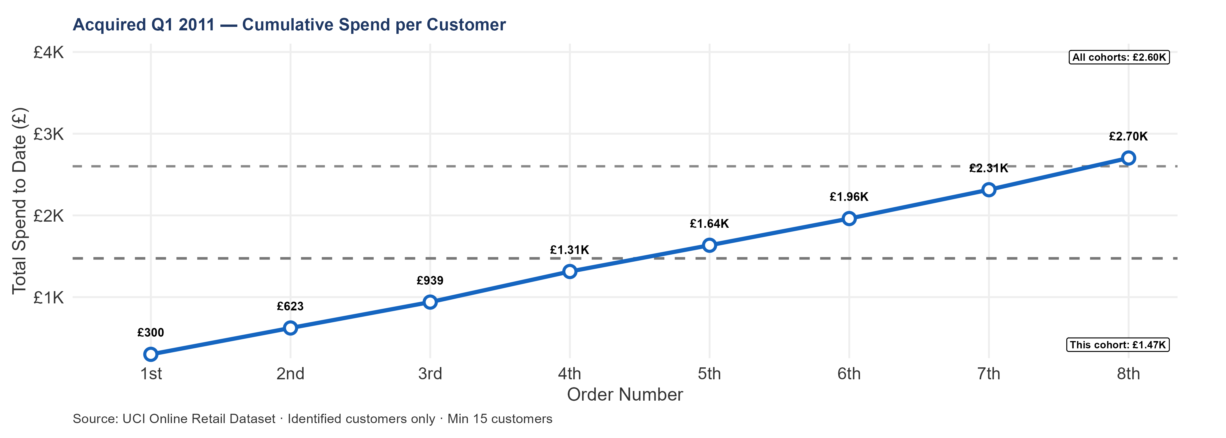
The Q1 2011 cohort is the largest acquisition quarter in the dataset — 1,248 new customers, 47.5% more than the Q3 2011 cohort. Cumulative spend per customer tracks below the all-cohort median. The acquisition volume and retention story for this cohort are the most important diagnostic in this section — detailed below.
6.5 Q2 2011 — Smaller Intake, Same Problem
Q2 brought in 826 new customers — a 34% drop from Q1, and without the silver lining a smaller pipeline could have hidden. Per-customer cumulative spend tracks below the dataset average, generating less per person than the larger Q1 cohort; both the volume and the quality of new customers declined at the same time.
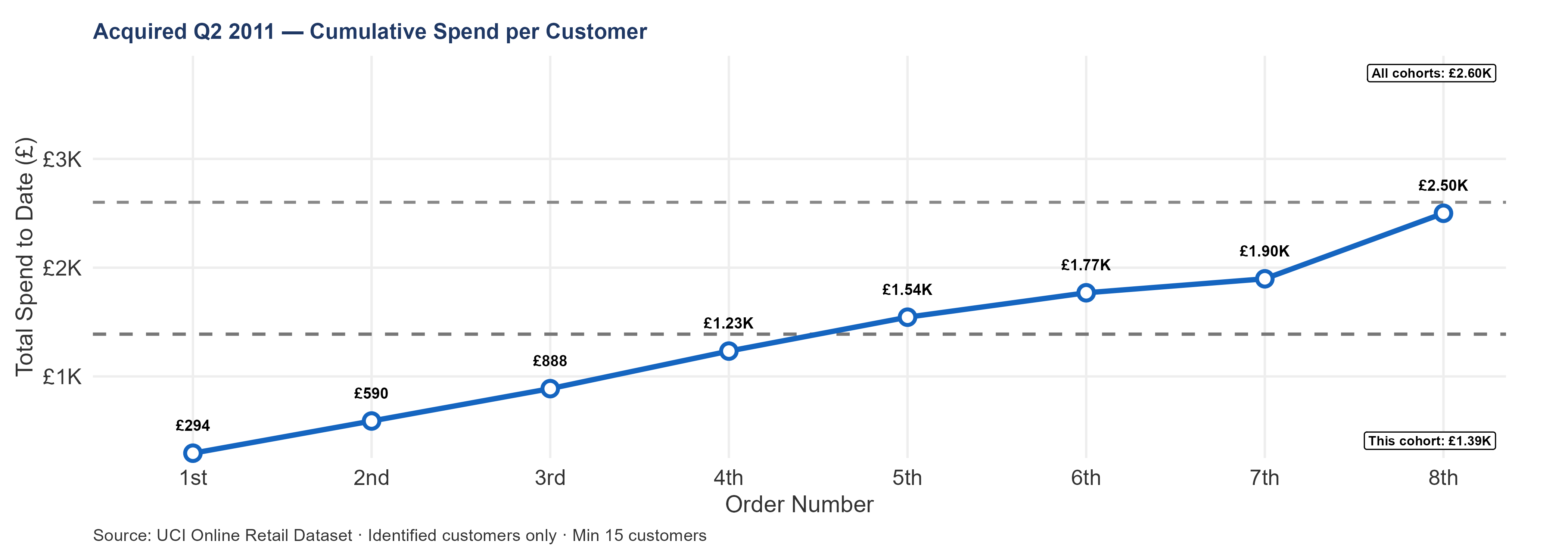
That joint decline rules out the most hopeful reading of Q1. If Q1’s retention problem had been a single bad campaign, Q2 — acquired through normal channels — should have rebounded to baseline; it did not. The persistence across quarters points toward a structural acquisition-quality issue rather than a one-off marketing misstep, and an acquirer modeling Q2 customers as a 2012 revenue source should apply a quality discount to this cohort.
6.6 Q3 2011 — The Summer Slowdown
Q3 was the quietest acquisition quarter — just 655 new customers, the smallest cohort of 2011 and the trough of the summer lull. Per-customer cumulative spend sits below the dataset average, continuing the downward drift that began in Q2.
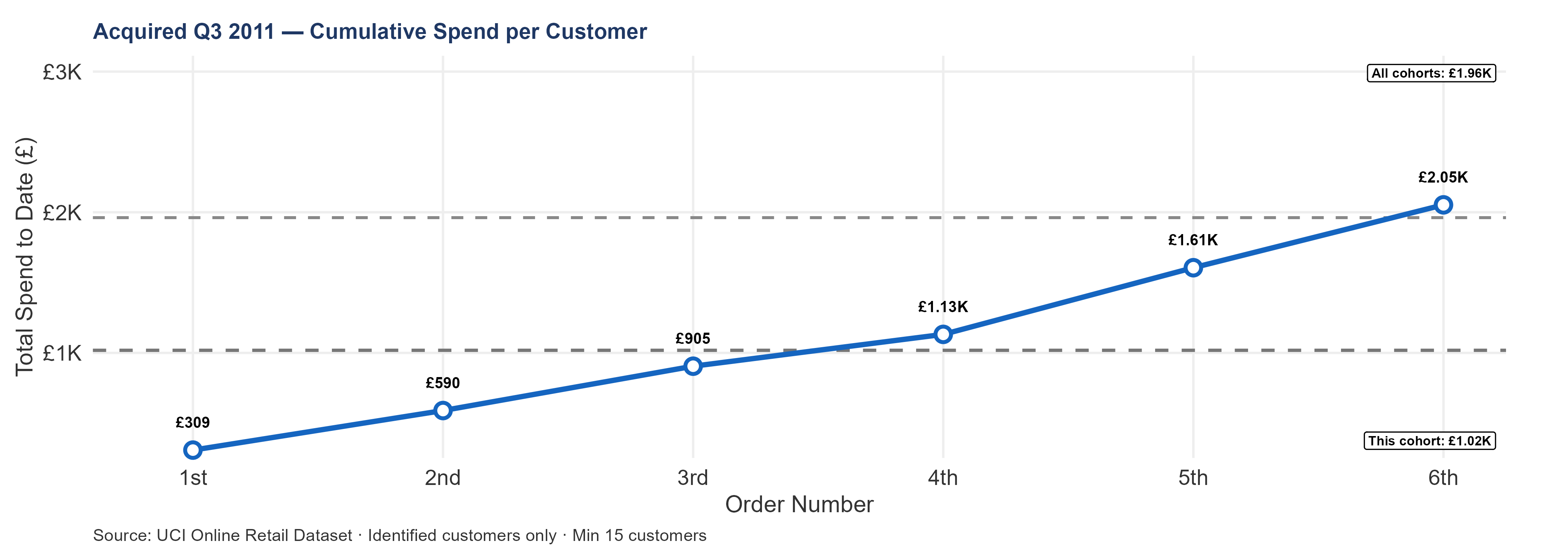
Q3 customers had a reasonable window to show early return behavior before the cutoff, so the below-average cumulative spend cannot be blamed entirely on the calendar; whether summer-acquired customers are inherently less committed or simply opportunistic is a question one year of data cannot answer. The forward revenue contribution from Q3 to 2012 is the smallest of any 2011 cohort by volume.
6.7 Q4 2011 — Too Early to Judge, Too Important to Ignore
The Q4 cohort is almost impossible to evaluate on retention. Customers acquired in October had two months of data at best. November arrivals had five weeks. December customers had days. Any retention chart for this group is measuring the calendar, not customer loyalty.
What Q4 does reveal is acquisition volume — and that number matters. Monthly new-customer counts recovered to 276–323 during the quarter, a meaningful bounce from the summer trough. It is not a full recovery to Q1 levels, but it shows the pipeline has not collapsed.
These customers are the wild card for 2012. They enter the new year with zero observable return history. Whether they come back at the historical rate of 65.46%, or at something lower, will only become clear from 2012 order data. An acquirer projecting Year 1 revenue should treat this as the single most important unknown in the dataset.
One thing is already certain: even if Q4 customers retain at the historical rate, the 2012 returning-customer pool will be smaller than 2011’s. Q1 2011’s massive 1,248-customer intake is not being replaced at equivalent volume. Any revenue model that assumes it will be is building on a pipeline that no longer exists.
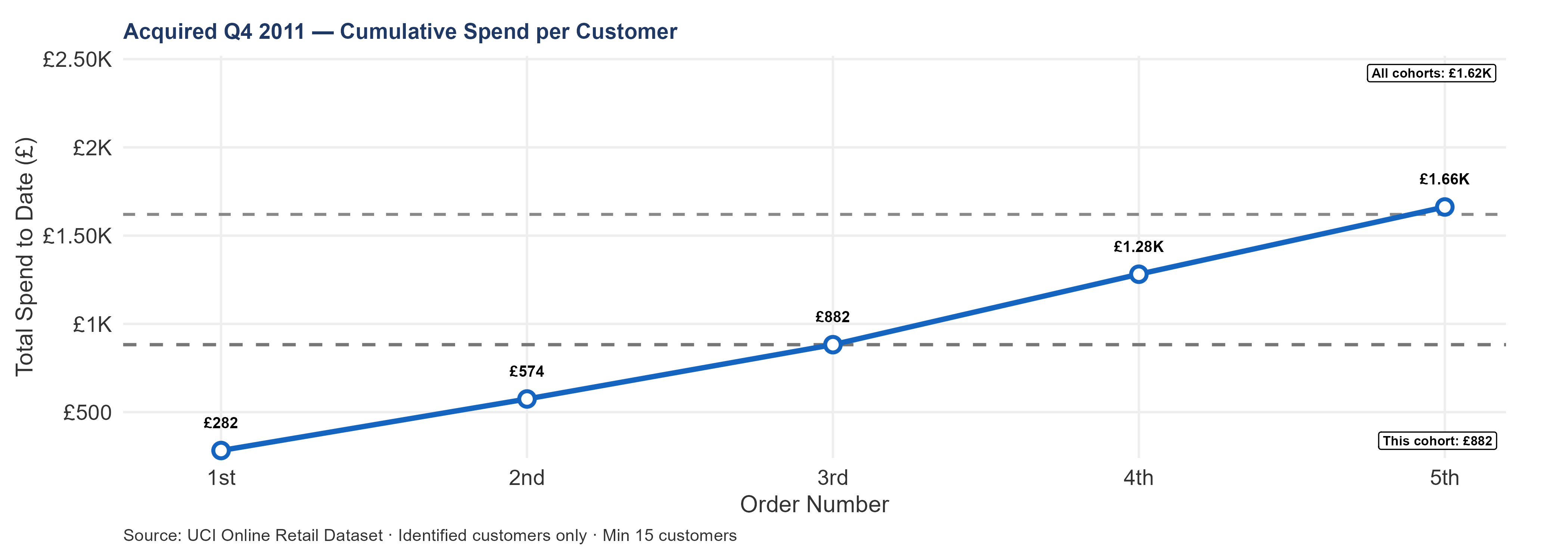
The Q4 2011 cohort covers customers acquired October through December 9 — the peak revenue quarter. This cohort is the most observation-truncated in the dataset: customers acquired in November had at most 5 weeks before the cutoff, and customers acquired in December had days. The chart shows almost no return order data for this cohort.
Critical caveat for the acquirer: Q4 2011 new customer acquisition (276–323 new customers/month in the recovery period) is the most important number in this cohort section for forward revenue modeling — not the cumulative spend curve, which is statistically unreliable at this observation window. These customers form the pool entering 2012 with zero prior return history. Their 1-to-2 retention rate — which will only be measurable from 2012 order data — is the single most important unknown for an acquirer projecting Year 1 post-close revenue. If Q4 2011 acquisition rates (276–323/month) hold into Q1 2012, and if those customers retain at the historical 65.46% rate, the 2012 returning-customer pool is substantially smaller than 2011’s — because Q1 2011’s 1,248-customer cohort is not being replaced at equivalent volume. Model this explicitly before setting 2012 revenue expectations.
6.8 Putting It All Together — Did Quality Fall Along with Volume?
All four 2011 quarterly cohorts are plotted together, with the solid gray line marking the dataset-wide average for customer spend over time.
The volume story is straightforward: 1,248 new customers in Q1, 826 in Q2, 655 in Q3, with a partial recovery in Q4. The business acquired fewer customers with each passing quarter through summer.
The quality story is what makes this uncomfortable. If the business were trading quantity for quality — acquiring fewer customers but better ones — the later cohorts would sit above the average line even as the earlier ones sat below it. They do not. Q1 shows the highest spending per customer of any 2011 group. Q3 tracks the lowest. The later cohorts are both smaller and no better per customer.
For an acquirer, this shapes the 2012 revenue picture in a concrete way. The 2012 returning pool draws from all four of these groups plus the December 2010 survivors. Q1 — the largest group by far, and the most uncertain in quality — will dominate. If Q1’s true retention is close to the December 2010 benchmark of 87%, the forward revenue numbers hold up. If Q1 genuinely retained at a lower rate, 2012 will fall short. Resolving this question is the single most valuable piece of analysis a buyer can do before signing.
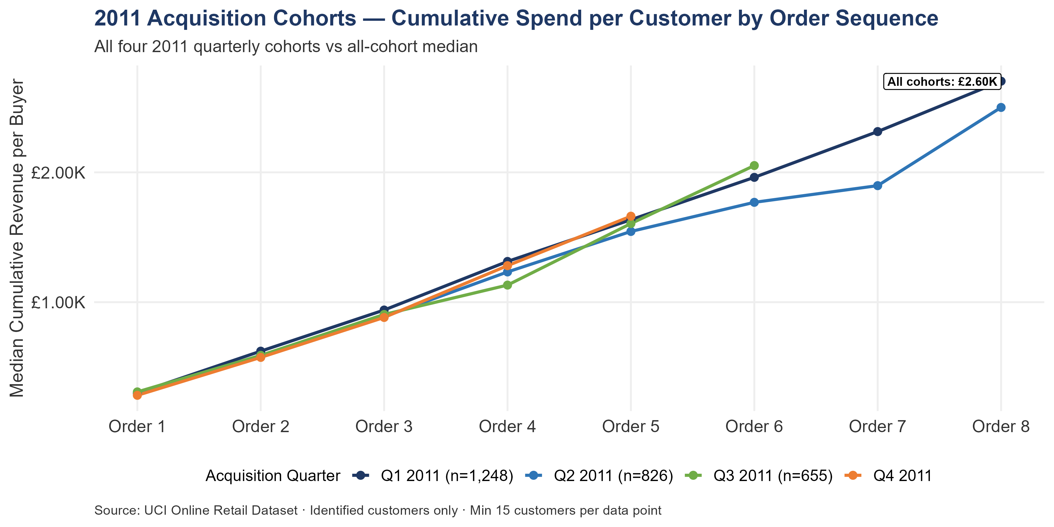
Acquisition volume fell through 2011 — but did customer quality hold?
The chart above places all four 2011 quarterly cohorts on the same axes. The solid gray line is the all-cohort median — the reference for average relationship quality across the full dataset.
Key observations:
Volume trajectory: Q1 (1,248 customers) → Q2 (826) → Q3 (655) → Q4 (recovering to 276–323/month). The business acquired fewer customers each quarter through summer, with a partial recovery in Q4.
Quality trajectory: The cohort with the highest median cumulative spend per customer is Q1 2011. The cohort tracking lowest against the all-cohort median is Q4 2011. Where a later cohort tracks above an earlier larger cohort, the volume decline was accompanied by quality improvement — fewer but better customers. Where a later cohort tracks below, both volume and quality declined simultaneously.
The 2012 returning-customer pool draws from these four cohorts. The Q1 2011 cohort (largest volume, most uncertain quality) will dominate the 2012 returning pool. If that cohort’s true retention rate is closer to the historical 65.46% than the observed truncated rate, 2012 returning revenue is defensible. If the cohort has genuinely lower quality than the December 2010 baseline, 2012 returns will disappoint. This is the single most important unknown in the dataset for 2012 revenue modeling.
The UK-specific view:
6.9 The UK Cohort View
The UK-specific heatmap confirms the pattern seen at the whole-business level. UK customers who are given enough time do come back at majority rates. What the business lacks is the infrastructure to make that happen systematically — a structured program that reaches out to new customers during the window when they are most likely to return.
For an acquirer building a UK revenue model, the Q1 2011 UK cohort is the right baseline — it has the longest observation window among 2011 groups and avoids the worst of the calendar distortion. If its retention rate, properly adjusted, approaches the December 2010 benchmark, the UK forward portfolio value in LTV Portfolio is well-supported. If it falls meaningfully short, that portfolio estimate needs to come down — and the Q1 investigation moves from useful to essential.
Did UK acquisition quality fall along with volume?
Among 2011 UK cohorts, Q1 shows the highest spending per customer. Q3 tracks lowest against the average. Where a later group spent more per person than an earlier one, the business was at least getting better customers even as it got fewer of them. Where a later group spent less, both volume and quality went down together.
The UK forward revenue projection depends on Q1 2011 customers retaining closer to the December 2010 rate than to the raw (truncation-distorted) 2011 numbers. Confirming this is the highest-value analytical task in the UK segment.

Q1 2011 — the largest UK cohort at 1,115 new customers — shows the steepest decay on the heatmap, confirming that the one-timer problem documented in Segmentation is structural rather than a small-cohort anomaly. Later cohorts had shorter observation windows: Q3 2011 customers had roughly three months before the December 9 cutoff, so their low off-diagonal retention partially reflects time truncation rather than genuine churn — interpret Q3 and Q4 2011 with that caveat, and do not treat them as LTV inputs. The Q1 cohort is the conservative forward-modeling baseline because it is the only 2011 group with a clean, full-window read of underlying retention.
UK Order-to-Order Transition Rates
Of 3,914 UK customers who placed at least one order:
- 1st → 2nd order: 2,562 customers returned (65.46% retention)
- 2nd → 3rd order: 1,819 customers returned (71.00% retention)
- 3rd → 4th order: 1,356 customers returned (74.55% retention)
The 1st-to-2nd transition at 65.46% is the single largest retention drop in the dataset. Every percentage point recovered at this transition produces more forward revenue than any other transition, because the customer pool is largest and the remaining LTV horizon is longest. Once a customer reaches their 3rd order, retention stabilizes — the 2nd-to-3rd and 3rd-to-4th transition rates are meaningfully higher than 1st-to-2nd. Getting customers from order 1 to order 2 is the most commercially valuable action in UK customer management.
On the December 2010 88% figure vs the 65.46% segment-wide rate: These measure different things. The 65.46% figure is the order-to-order transition rate across all UK customers in the dataset, including those acquired late in 2011 who had only 1–3 months to return before the December 9 cutoff. The 88% December 2010 cohort figure is a 12-month window retention rate for a single cohort with a full year to either return or not. They are not contradictory — they describe different populations with different observation windows.
Owner: buyer’s UK commercial lead. Action: within Month 1 (Days 1–30) of close, confirm whether the day-30 first-order follow-up program targets all UK first-time customers or only those matching the Q1 2011 cohort profile (which showed the steepest decay). Decision determines program scope and budget.
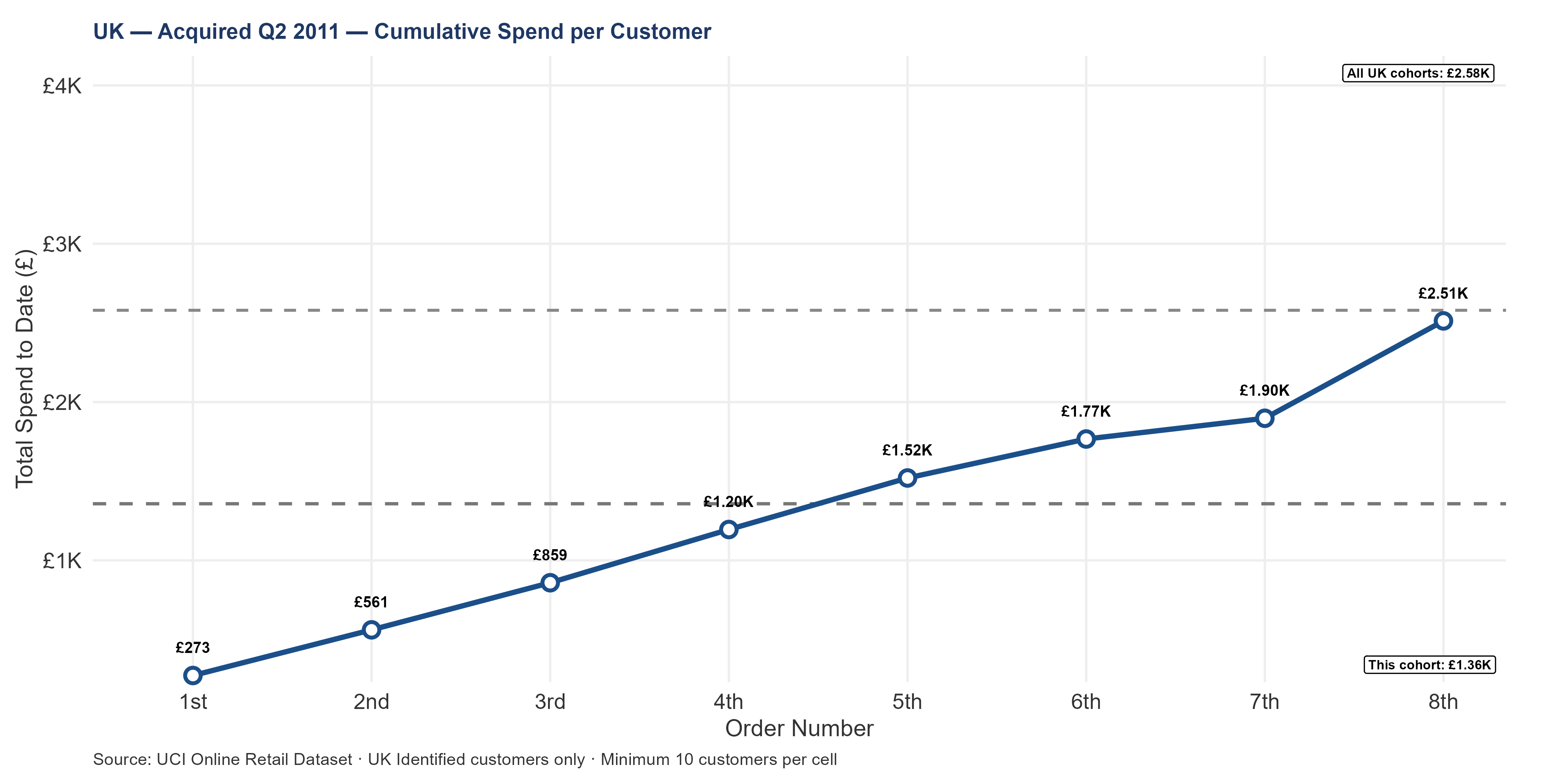
6.9.1 UK Customer Lifetime Value by Acquisition Cohort
Each chart tracks one cohort’s cumulative spend per customer from order 1 through order 8. The gray dashed line is the UK-wide median across all cohorts. A cohort sitting above it has more valuable customers than average; below it, less.
The telling distinction is between a cohort that starts above the median and stays there — genuine relationship depth — and one that starts above but drifts back by order four or five, suggesting inflation from a few large early purchases. That gap separates a good acquisition quarter from a lucky one.
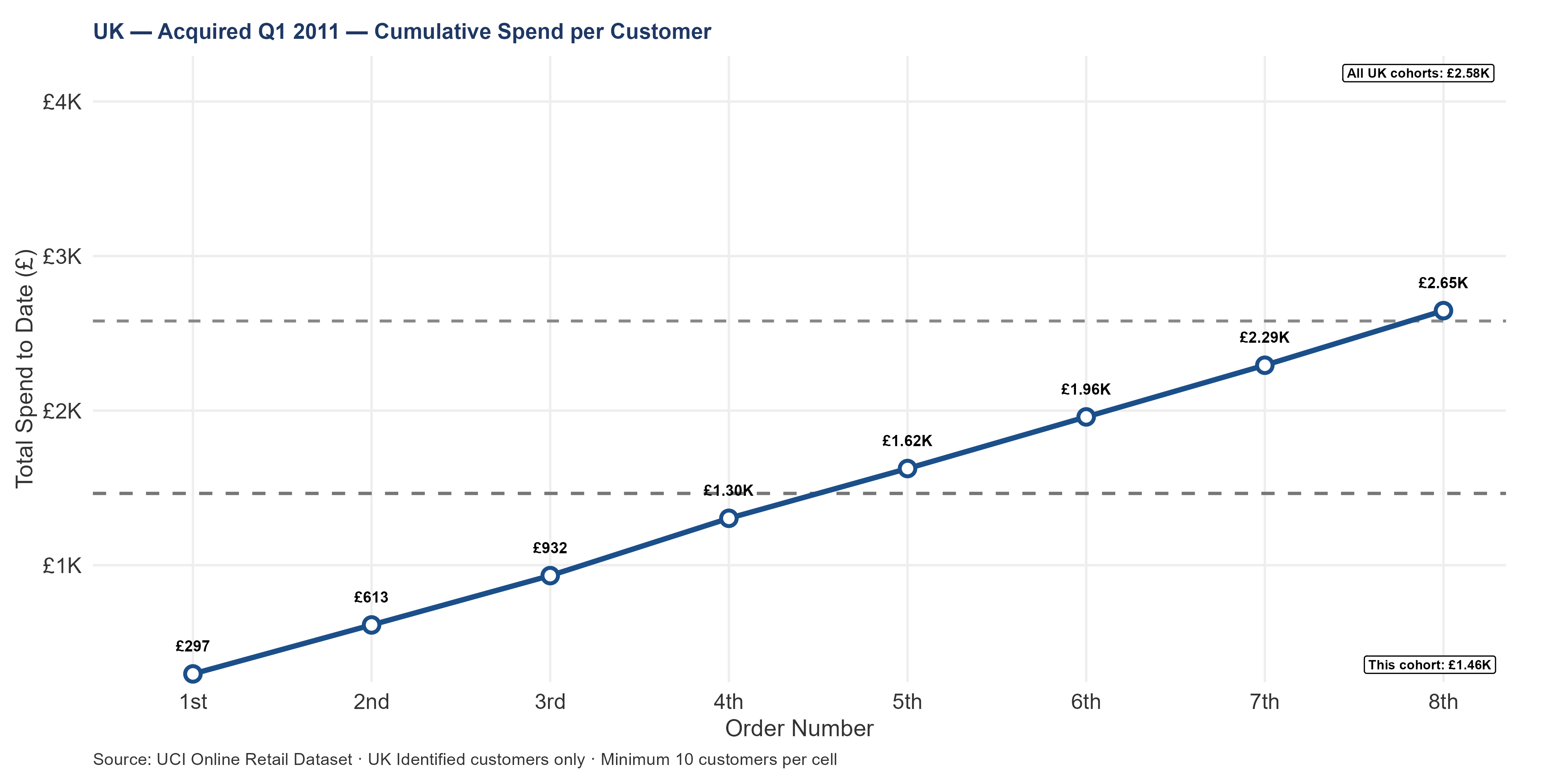
6.9.2 Q1 2011 — The Largest UK Cohort
Q1 2011 produced 1,115 new UK customers — the single largest acquisition quarter in the UK segment. Volume alone makes this group the most consequential for forward revenue. But volume and value are separate questions. A large cohort that churns quickly can generate less total revenue than a smaller one where customers keep coming back.
Q1 customers sit relative to the UK median at each order number. Whether the gap widens, holds steady, or closes as orders accumulate determines whether this cohort’s early performance was durable or front-loaded.
A Q1 line consistently above the median means these customers are both numerous and individually valuable — the strongest possible 2012 revenue signal. A line converging back toward the median by order five or six suggests early-order inflation (promotional pricing, large initial stocking orders) with underlying relationship quality no different from the rest of the base.
Q1 2011 will contribute more customers to the 2012 returning pool than any other group. Whether those customers compound value at, above, or below the UK median directly determines whether the forward portfolio estimate is conservative, accurate, or optimistic.
Warning
Q1 2011 UK Cohort — Largest Acquisition Quarter, Highest One-Timer Rate: Investigate Before Repeating
Q1 2011 produced the most new UK customers (1,115) and the highest observed one-time-customer rate among cohorts with enough data to measure reliably. The combination of high volume and high churn is the most commercially important diagnostic in the UK cohort data.
Two explanations fit the evidence equally well, and the data alone cannot distinguish between them.
Explanation A — the observation window. Q1 customers had at most nine months before the dataset’s December 9 cutoff. Customers whose natural buying cycle falls on a ten-, eleven-, or twelve-month rhythm would be counted as one-timers even though they were always going to come back. If this is what happened, the true retention rate is much better than it appears.
Explanation B — acquisition quality. Something about Q1 2011 acquisition — a promotional campaign, a new channel, a pricing change — attracted customers who were never likely to become repeat wholesale accounts. If this is even partially correct, repeating the same approach in Q1 2012 means repeating the same expensive experiment with the same uncertain outcome.
The investigation question: what was different about how the business acquired customers in Q1 2011?
6.9.3 Q2 2011 — Did the Smaller Intake Produce Better Customers?
Q2 brought in fewer customers than Q1 — a natural step-down from the year’s peak. Whether the business traded volume for quality is the question. A smaller cohort tracking above the UK median means the pipeline self-selected for better customers as it narrowed. Tracking at or below the median means fewer customers without better ones.
Where Q2 sits relative to Q1 across the order sequence also illuminates the Q1 investigation. If Q1’s weak retention stemmed from a one-off bad campaign, Q2 — presumably acquired through normal channels — should bounce back to baseline quality. If Q2 also underperforms, the quality problem extends beyond Q1 and may be structural.
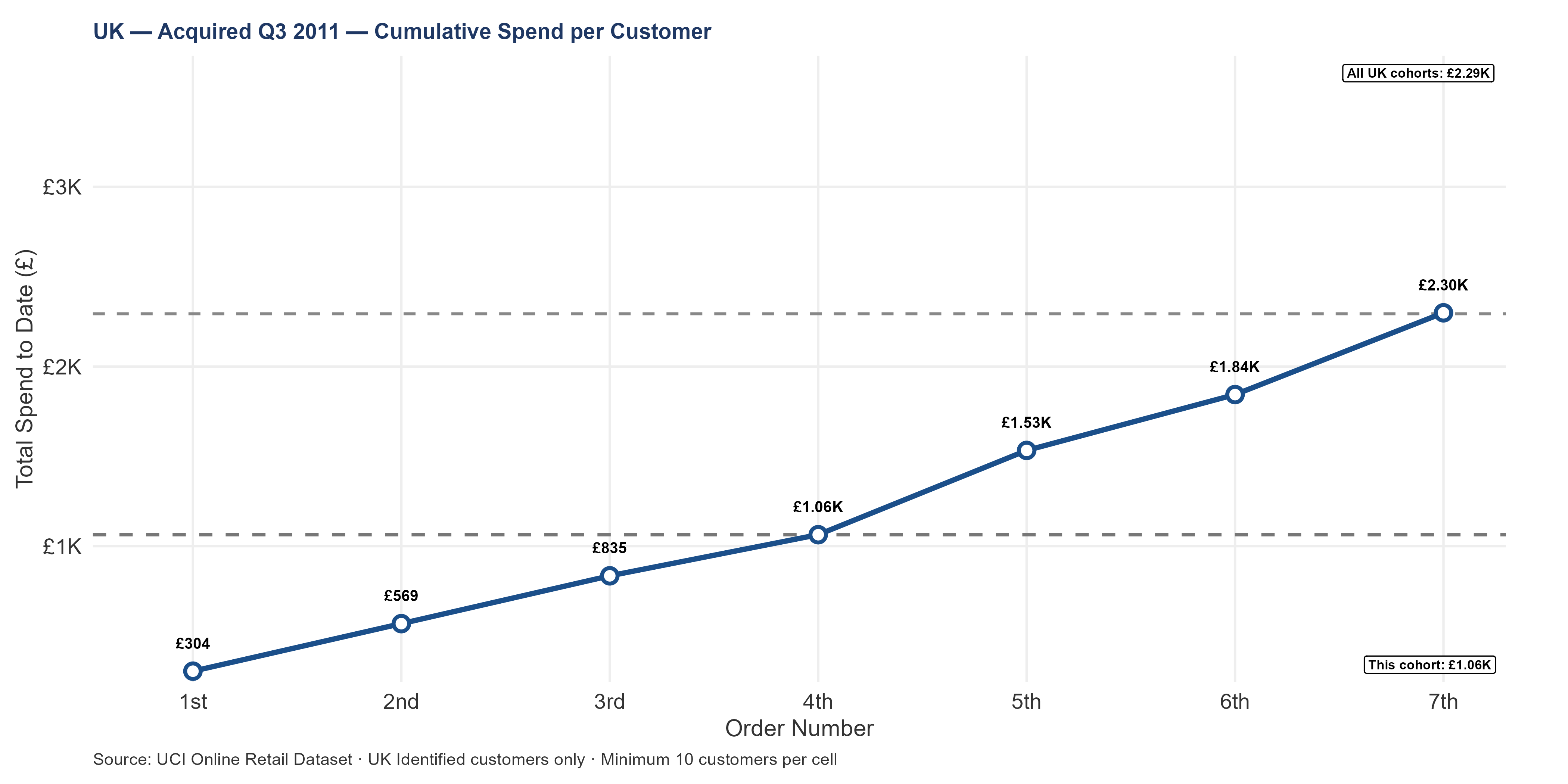
6.9.4 Q3 2011 — The Summer Cohort
Q3 was the quietest acquisition quarter — 655 new UK customers, coinciding with the summer wholesale lull. Whether summer-acquired customers behave differently is the question.
If Q3 customers track above the UK median on their own merits, summer acquisition is quietly producing better-than-average relationships. If they track below, the summer trough is a quality problem as well as a volume one. The slope of Q3’s cumulative-spend line relative to Q1 and Q2 shows whether these customers compound value faster, slower, or at the same rate — the steepest slopes belong to the cohorts with the strongest long-term relationships.
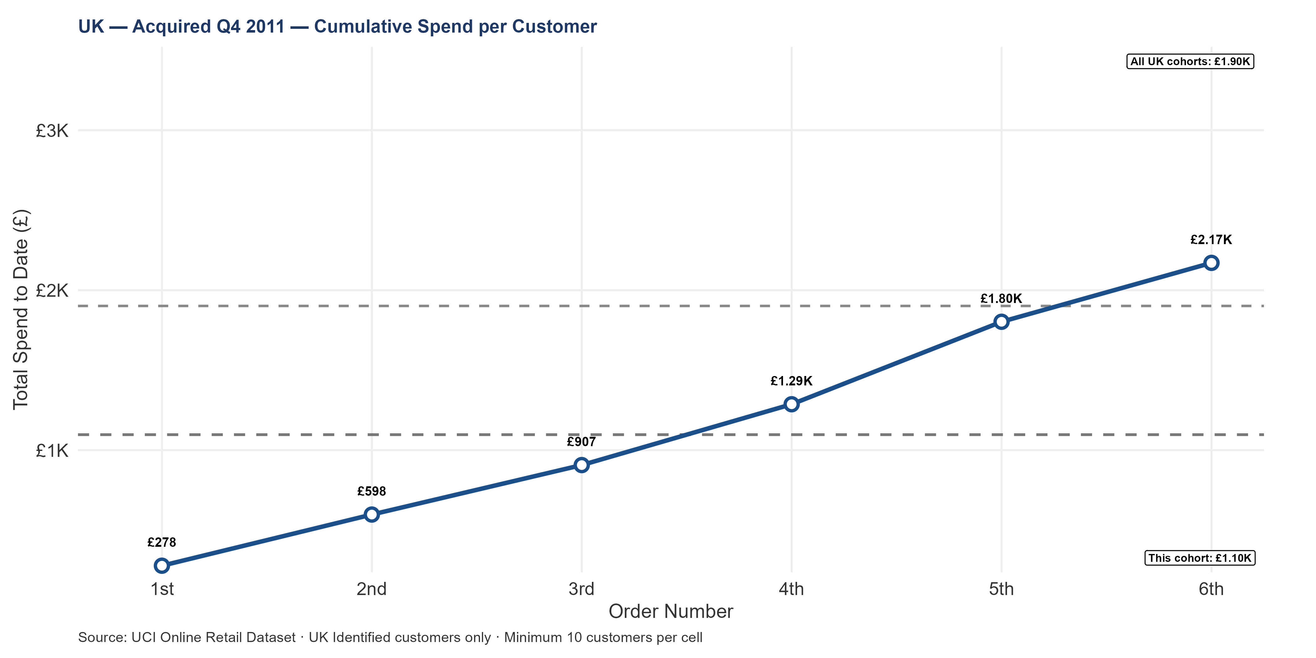
6.9.5 Q4 2011 — Insufficient Observation Window
The Q4 cohort entered the dataset between October and December 2011, leaving at most a two-month observation window for the earliest arrivals and as little as a single month for the latest. That truncation makes any spending trajectory mechanically determined by the calendar rather than by actual purchasing behavior. This cohort should be excluded from trend interpretation on this chart.
6.9.6 All 2011 UK Cohorts Together — The Full Picture
All four 2011 UK quarterly cohorts are overlaid against the UK-wide median. Among them, Q1 shows the highest median cumulative spend per customer. Q3 — the summer cohort — tracks lowest: fewest customers and least valuable per person.
Whether the lines converge or diverge over time reveals the trajectory. Convergence toward the median by later cohorts means the business acquired progressively weaker customers as the year went on. Roughly parallel lines mean per-customer quality held even as volume fell. Where a later cohort tracks above an earlier one at the same order number, the business was getting better customers even as it got fewer — a reassuring sign. Where a later cohort tracks below, both volume and quality declined together.
The UK forward revenue projection depends on Q1 2011 — the largest cohort by volume — retaining closer to the December 2010 baseline than to the truncation-distorted 2011 measurements. Confirming which scenario applies is the highest-value analytical task in the UK segment.
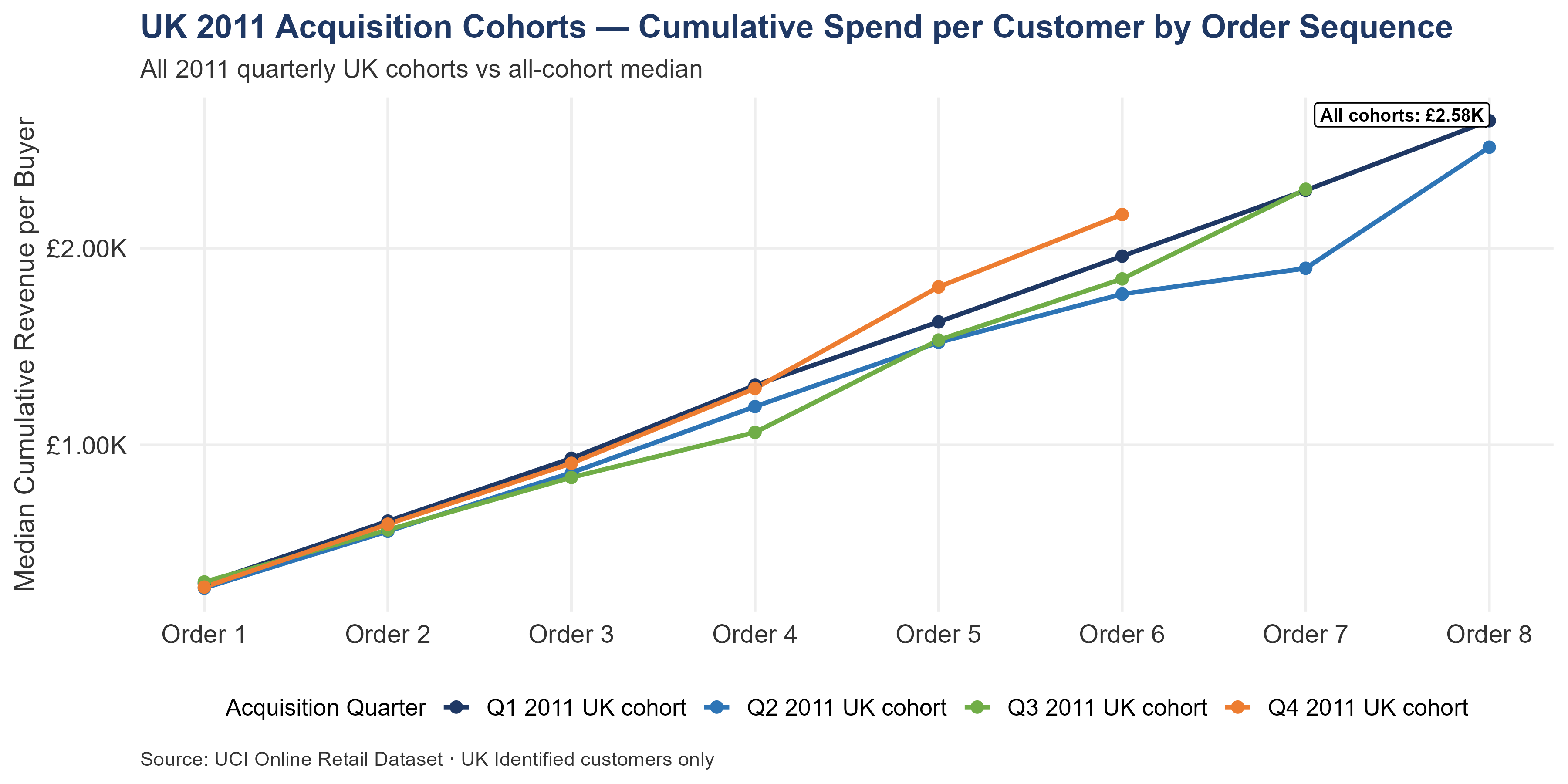
Among 2011 UK cohorts, the highest median cumulative spend per customer belongs to Q1 2011; the lowest tracker against the all-cohort median is Q3 2011. Where a later cohort tracks above an earlier one, UK acquisition was getting better per customer even as volume fell; where it tracks below, both volume and per-customer quality declined together.
The navy line tracks cumulative spend per UK customer from order 1 through order 8; the gray dashed line is the UK overall median. A steep slope means the cohort compounds value quickly. A cohort that starts above the median and returns to it by order 8 may have been boosted by a single large early order — genuine relationship depth requires the line to hold above the median consistently.
A UK customer who reaches their 8th order has generated £2.58K in cumulative median revenue. This is an observed historical figure. The forward LTV for a new UK customer — probability-weighted by the risk that many will not return for a second order — is £1.24K at 3 years. This figure accounts for churn: it multiplies the per-retained-customer LTV by the probability of retention at each step, producing a lower expected value than what a retained customer actually generates. The full LTV methodology and parameter choices are in LTV Methodology. For Q1 2011 cohort of 1,115 customers:
- 1% improvement in 1st-to-2nd retention: That improvement retains roughly 11 additional customers, each generating approximately £1.23K in forward LTV beyond order 1. Value per percentage point: approximately £13.76K.
This is why the day-30 follow-up program — targeting the 1st-to-2nd transition — is the highest per-customer value intervention available to the UK account team. The customer pool is at its largest and the remaining LTV horizon is at its longest at exactly this transition.
6.10 The International Cohort View
International cohort retention follows the same general shape as the UK, with one important difference: the numbers are less statistically reliable. International cohorts are smaller, which means individual accounts carry outsized influence. A single large international customer going quiet can move a quarterly retention figure by several percentage points. The confidence around any international cohort rate is wider than its UK equivalent.
Among 2011 international cohorts, Q2 shows the highest spending per customer. Q4 tracks lowest. The international segment’s cancellation rate — which doubled between H1 and H2 — adds a complicating layer. Whether the customers acquired during the higher-cancellation period also show lower per-customer value would reveal whether the H2 deterioration was a narrow operational hiccup or part of a broader quality problem.
How international customers deepen over time
Of 414 international accounts that placed at least one order, 262 came back for a second (63.29%). Of those, 179 returned for a third (68.32%), and 140 for a fourth (78.21%). The pattern is clear: each successive order makes the next one more likely. Customers who survive the first-to-second hurdle become progressively stickier.
That first hurdle is the one that matters most. The drop from 100% to 63.29% at the first-to-second transition is the steepest in the entire sequence. Every percentage point recovered at this stage produces more future revenue than improvement at any other point — because the pool of accounts is largest and the remaining years of potential spending are longest. At the international segment’s median order value of £391 — 1.3 times the UK median — each account that crosses this threshold is worth meaningfully more than a UK conversion.
What each percentage point is worth
A single percentage-point improvement in first-to-second international retention saves roughly four additional accounts. Each generates approximately £809 in forward value beyond their first order. That works out to about £3.35K per percentage point — 1.3 times higher than the equivalent UK figure.
The day-30 follow-up program targets precisely this transition. Its per-account payoff is higher in the international segment than anywhere else in the business.
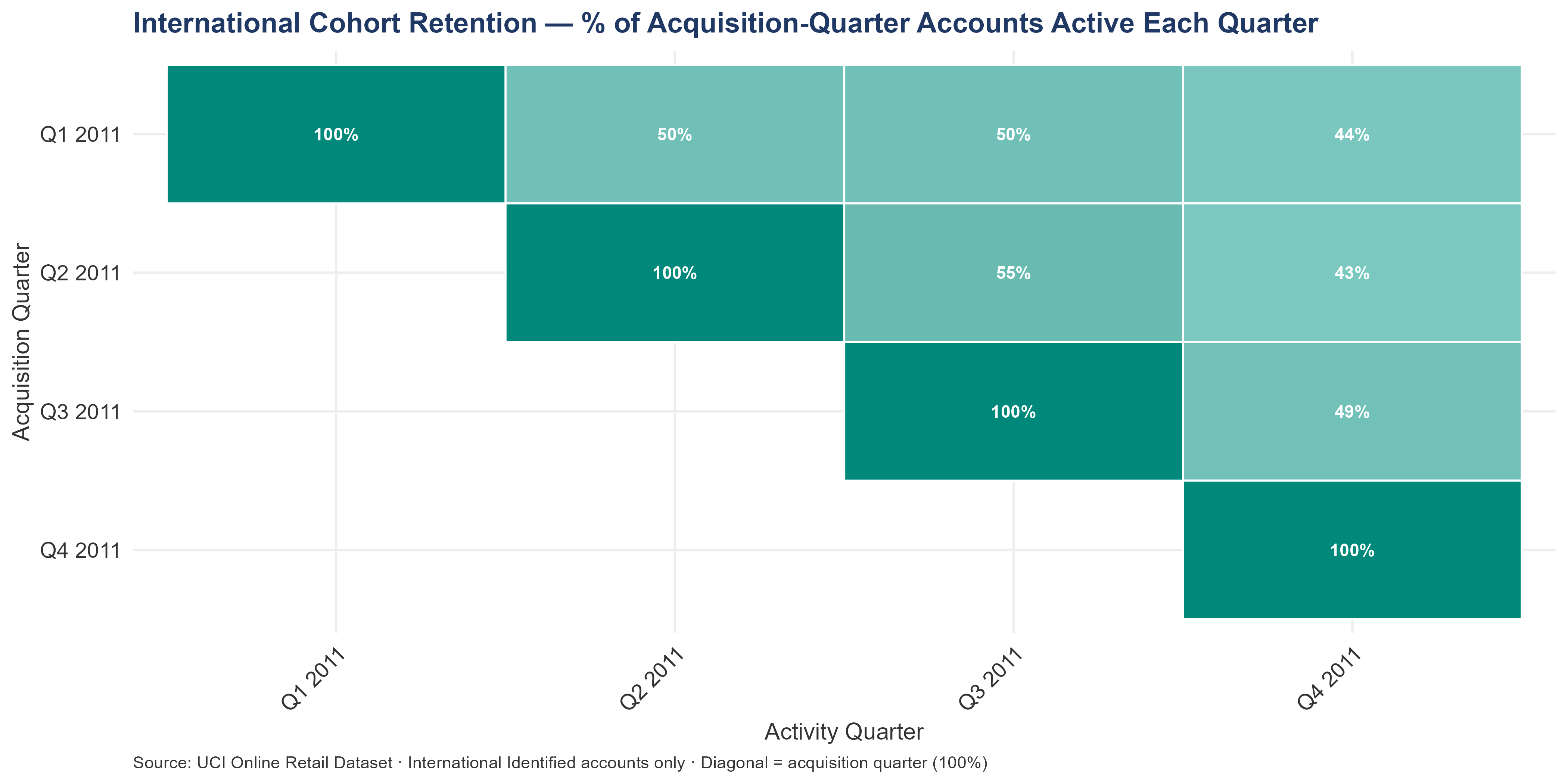
Use the Q1 2011 international cohort as the forward-modeling baseline: it has the longest observation window in the dataset and avoids truncation bias. Q3 2011 international accounts had only about three months before the December 9 cutoff, so their low off-diagonal retention reflects window truncation as much as genuine churn — interpret Q3 and Q4 with that caveat rather than treating them as LTV inputs.
International Order-to-Order Transition Rates
Of 414 international accounts that placed at least one order:
- 1st → 2nd order: Of the full base, 262 accounts returned (63.29% retention)
- 2nd → 3rd order: Of those, 179 accounts returned (68.32% retention)
- 3rd → 4th order: Of those, 140 accounts returned (78.21% retention)
The 1st-to-2nd transition at 63.29% is the single largest retention drop. Every percentage point recovered at this transition produces more forward revenue than any other transition, because the account pool is largest and the remaining LTV horizon is longest. At the international segment’s median AOV of £391 — 1.3× the UK median — each converted account is worth materially more than a UK conversion. Getting international accounts from order 1 to order 2 is the most commercially valuable action in international customer management.
International Landscape identified 72 international accounts that were active in H1 2011 and went silent in H2 — combined H1 revenue £52.63K. These are not new one-timers; they are established accounts that made a first-to-second or subsequent transition, then lapsed before Q4. The retention program for these accounts is reactivation (not first-time conversion), and the Segment Programs international outreach script applies. Treat these 72 accounts as a higher-priority list than the one-time conversion pool.
The buyer’s International commercial lead should, within Month 1 (Days 1–30) of close, confirm whether the day-50 first-order follow-up trigger targets all new international accounts or only those matching the Q1 2011 cohort profile. Decision determines program scope.
6.10.1 International Customer Lifetime Value by Acquisition Cohort
Which international acquisition cohorts compound value fastest — and how does the trajectory change?
Each chart shows one acquisition cohort’s cumulative median spend per account as they place their 1st through 8th order. The gray dashed line is the overall international median across all cohorts — the baseline for comparison.
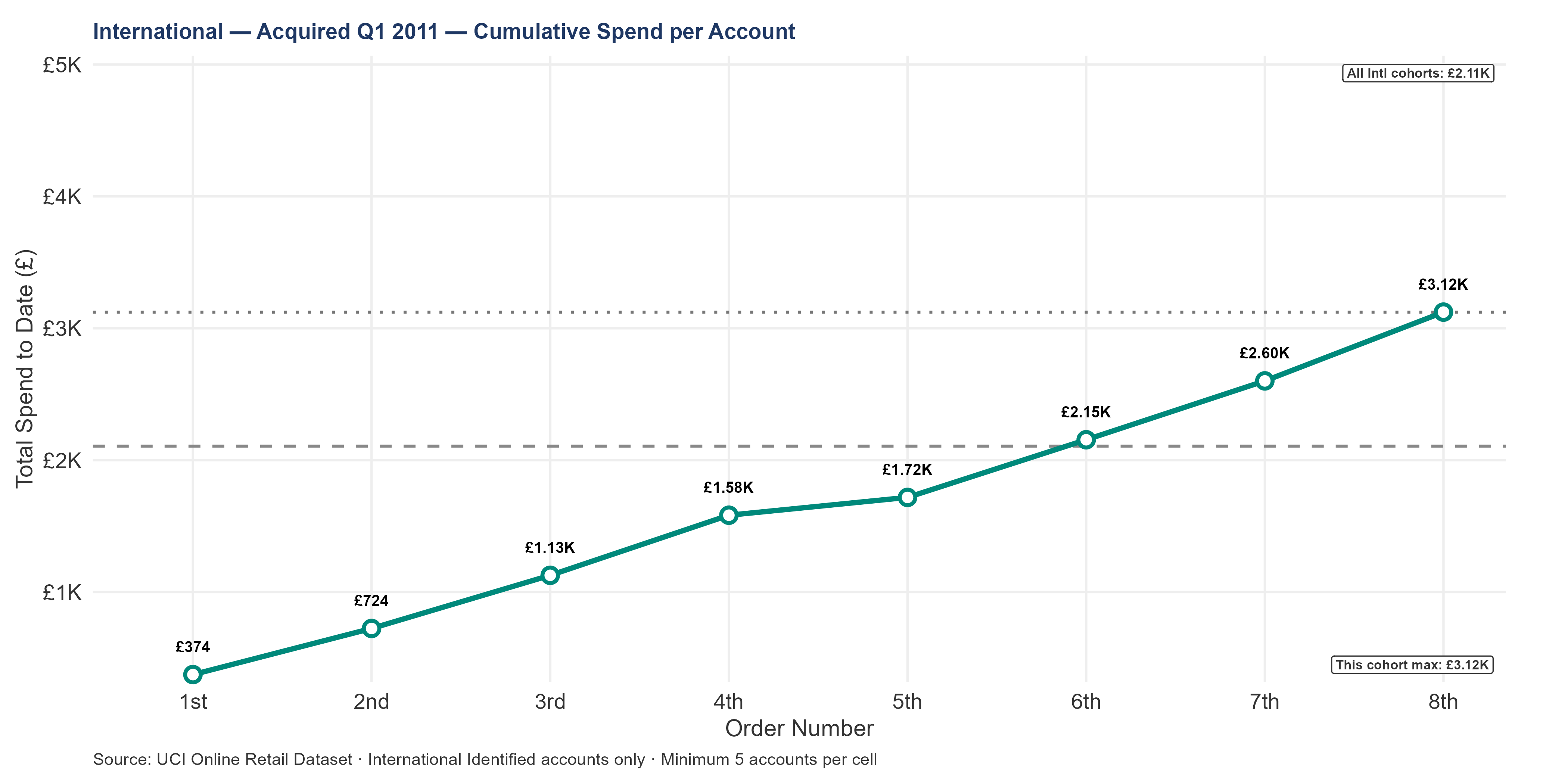
The Q1 2011 international cohort acquired 132 new accounts. This is the earliest 2011 cohort with a full multi-quarter observation window. How its LTV curve compares to the gray median determines whether early-2011 acquisition produced above-average or below-average international relationships.
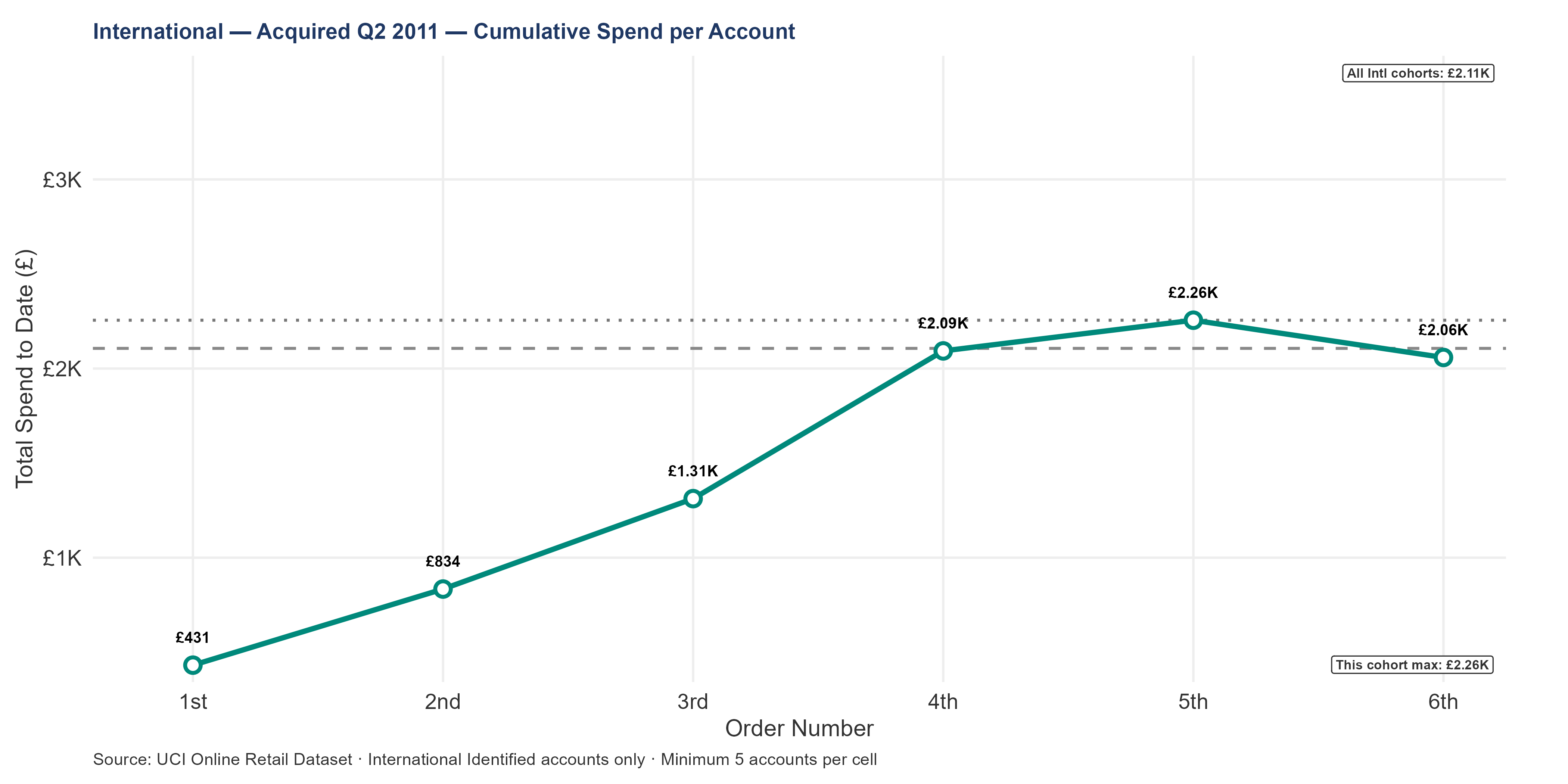
The Q2 2011 international cohort acquired 77 new accounts. Compare the slope of this cohort’s LTV curve against earlier cohorts to assess whether acquisition quality is improving, stable, or declining over time.
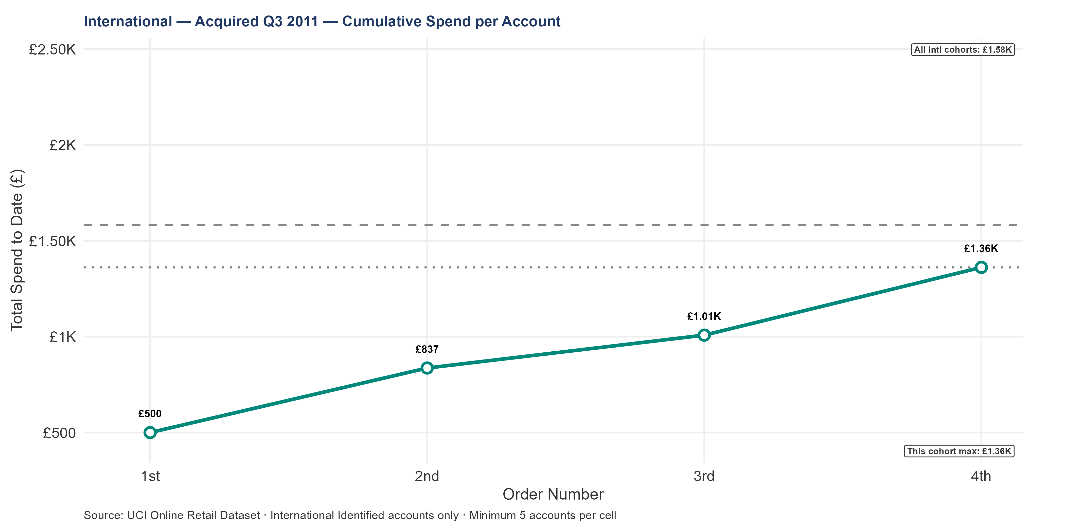
The Q3 2011 international cohort acquired 68 new accounts. Compare the slope of this cohort’s LTV curve against earlier cohorts to assess whether acquisition quality is improving, stable, or declining over time.
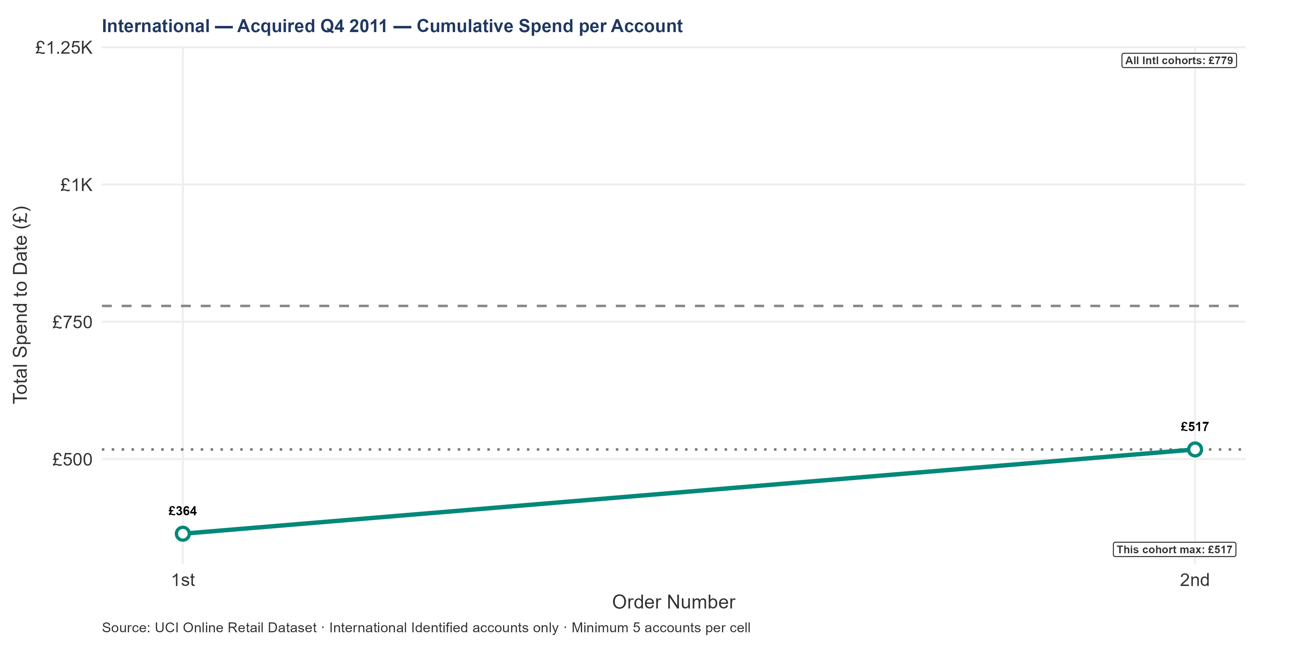
The Q4 2011 international cohort acquired 67 new accounts. This is the most recent cohort — accounts acquired in the final weeks of the analysis period. They have had almost no time to demonstrate a reorder pattern. Whether they return will become clear in Q1 2012.
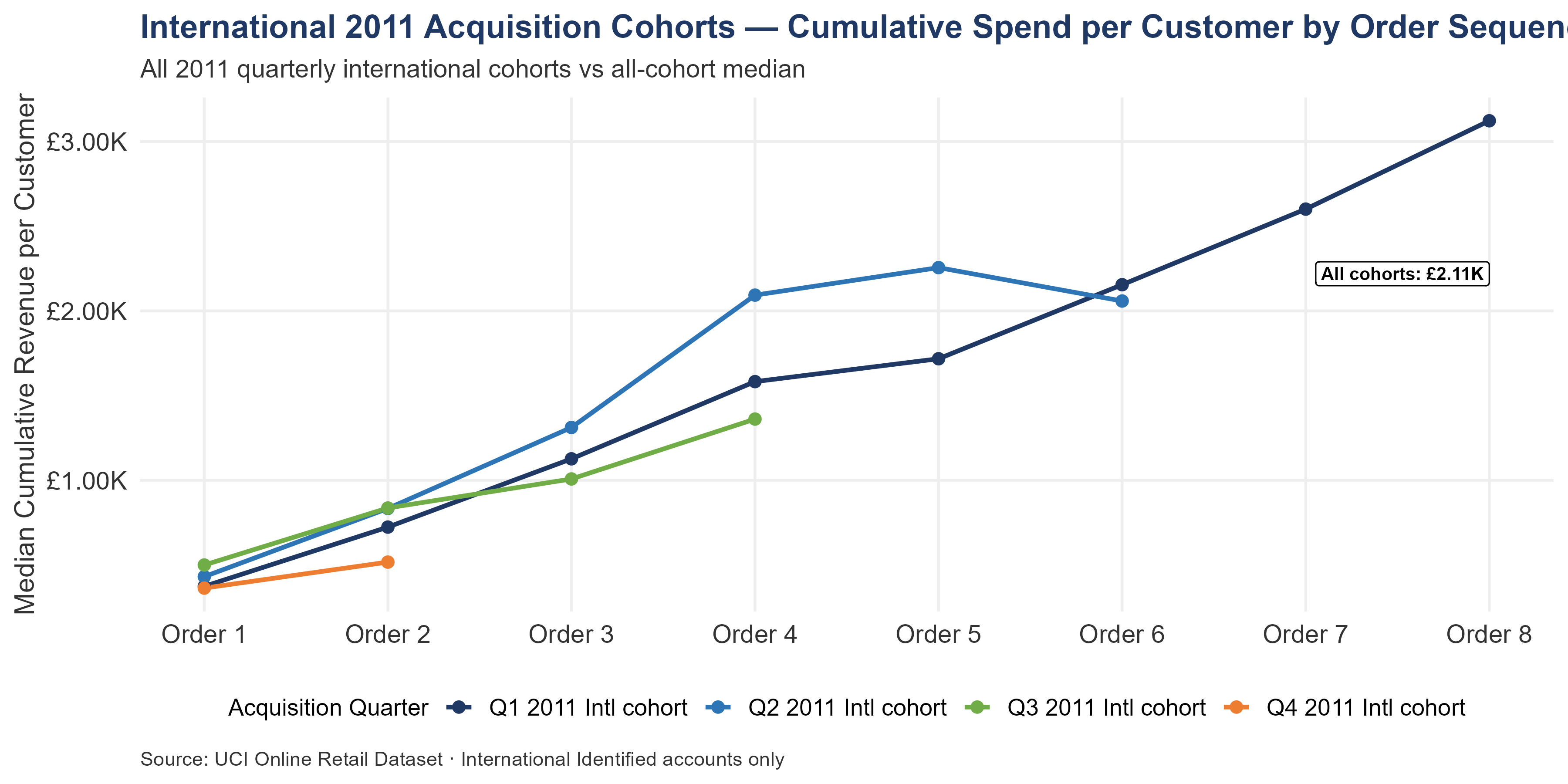
The chart above overlays all 2011 international quarterly cohorts on a single axis to assess quality trajectory across the year.
The solid gray line is the international all-cohort median — the reference for average international relationship quality.
Among 2011 international cohorts, the highest median cumulative spend per customer belongs to Q2 2011. The cohort tracking lowest against the all-cohort median is Q4 2011. The international segment’s H1-to-H2 cancellation rate doubling is the primary concern for this segment; read the 2011 cohort quality trajectory against that context — whether the cohorts acquired in the deteriorating cancellation period also show lower per-customer cumulative spend determines whether the H1/H2 shift reflects a narrow operational issue or a broader acquisition-quality problem.
An international account that reaches its 8th order has generated approximately £2.11K in cumulative median revenue. The forward LTV for a new international account — probability-weighted by the risk that many will not return for a second order — is approximately £1.59K at 3 years. This is the new-account expected value; it accounts for churn. Appendix A §A.7 documents the steady-state ceiling at approximately £3.68K International under higher long-run retention assumptions. That figure is a methodological ceiling sensitivity, not the preferred base case; the chain-model figure above is the authoritative value for acquisition financial modeling.
A 1% improvement in 1st-to-2nd retention saves approximately 4 additional accounts, each generating approximately £809 in forward LTV beyond order 1 — a value per percentage point of approximately £3.35K.
At the international segment’s median AOV of £391, this per-point value is 1.3× higher than the equivalent UK figure. The day-30 follow-up program — targeting the 1st-to-2nd transition — has a higher per-account payoff in the international segment than in any other segment.
Author: Shawn Phillips | Lailara LLC
← International Customer Landscape | Conversion Windows & Reorder Intervals →